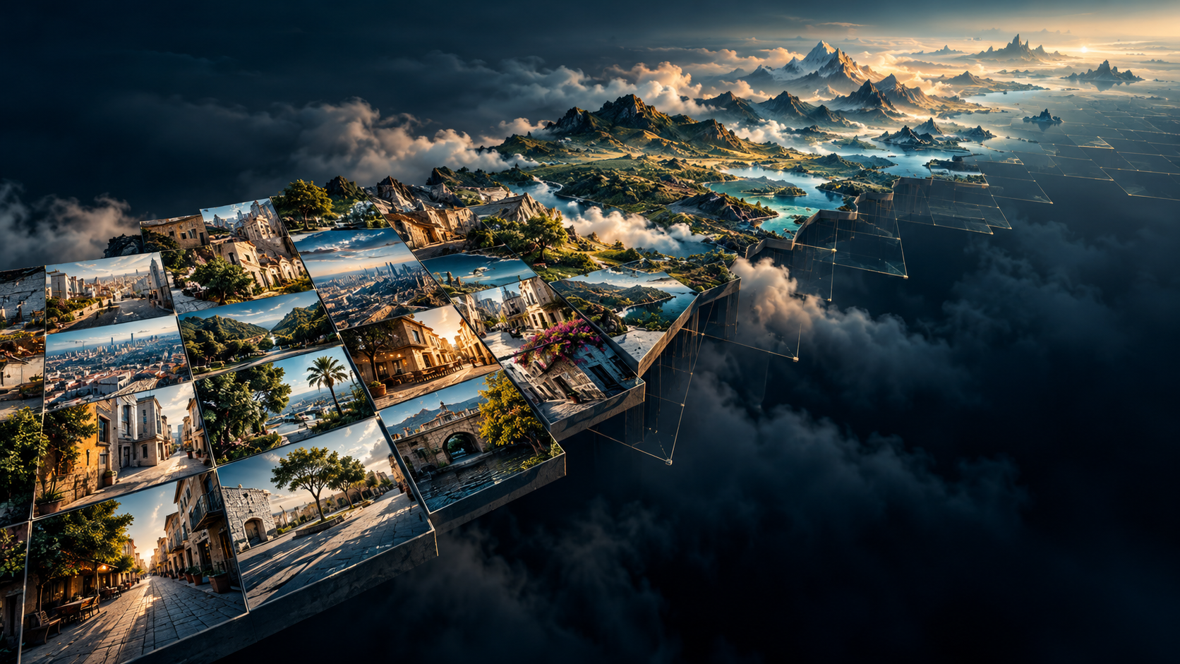
Ask an image generator for an ordinary street in a specific town. It may produce convincing buildings, vegetation, vehicles and people. The scene can look like a photograph without establishing that those things exist together in that town.
This raises a question beyond image quality: when does a model reproduce place-specific information, and when does it complete missing information with a plausible visual pattern?
We built an interactive program to investigate a measurable precursor: the mismatch between where people live and where photographs are recorded. Its map measures representation in a historical dataset. Whether those imbalances predict a particular model’s errors remains a separate experiment.
Explore the photographic representation map
Switch between population, Flickr frequency and their relative difference. Select a cell to inspect its population, recorded contributions and population-proportional expectation. Regional views make the individual cells easier to see.
The blue–orange layer answers a precise question: does this cell account for a larger or smaller share of recorded contributions than its share of population? It is not a map of intelligence, cultural importance or proven AI ignorance.
Population, photographs and information are different quantities
A populated region offers many potential image producers. That does not guarantee that their pictures reach a particular public platform, retain geographic coordinates or enter a model’s training corpus. A sparsely populated destination can attract visitors who collectively produce enormous numbers of photographs.
Even counting photographs leaves another gap. Ten thousand near-identical landmark views can contain less varied information about everyday life than a smaller collection covering residential streets, workplaces and markets. That is an illustration of redundancy, not a measured comparison in this project.
The distinction is fundamental:
Population density ≠ photographic frequency ≠ informational diversity.
Our first map deliberately measures the relationship between the first two. Diversity and semantic coverage need additional measurements.
How the program calculates the delta
The photographic layer comes from Dunkel, Löchner and Burghardt’s published YFCC100M grid-aggregation work . The underlying YFCC100M collection covers Flickr uploads from 2004 to early 2014 and includes photos and videos. Accordingly, the program labels its counts Flickr contributions, rather than claiming to count every photograph of Earth.
We pair that historical snapshot with GHS-POP R2023A , using its modelled residential population for 2010. The source population grid has 1-km cells. Summation resampling transfers those values to the original 100 × 100 km Mollweide grid, preserving the distinction between counts and densities. Each full projected cell covers 10,000 km².
For every eligible cell, the calculation is:
expected contributions = cell population × total contributions / total population
representation ratio   = observed contributions / expected contributions
map delta              = log2(representation ratio)
Both totals refer to the same reference domain: cells with available contribution counts and at least 100 residents. Proportionality is a comparison baseline, not a claim that everyone should produce the same number of pictures.
| Ratio | Log₂ delta | Interpretation |
|---|---|---|
| ¼ | −2 | One quarter of the population-proportional expectation |
| 1 | 0 | Contribution share matches population share |
| 4 | +2 | Four times the expectation |
Blue encodes lower representation; orange encodes higher representation. The colour scale saturates at 1/64 and 64 times the expectation, while cell details retain the actual factor. Violet marks a recorded count of zero. Missing counts and cells with fewer than 100 residents receive no ratio. No artificial extra contribution is added to make zero counts logarithmically convenient.
What this first calculation shows
After exclusions, the reference domain contains 13,316 cells, approximately 47.68 million contributions and 6.98 billion modelled residents. These are sums in this analysis, not estimates of today’s population or photographic activity.
The map makes the uneven distribution visible. Much of Europe and the United States appears above the population-proportional benchmark, while many cells in Africa and South Asia appear below it. This describes the selected Flickr snapshot; it does not characterize the total visual knowledge available in those regions.
For a concrete example, the 100-km cell near Lagos, centred at approximately 6.7° N, 3.1° E, contains about 12.72 million modelled residents and 1,037 recorded contributions. Its proportional expectation is approximately 86,845: about 84 times the observed count. The cell is not the administrative boundary of Lagos, and that factor says nothing directly about an image generator’s accuracy there.
There is an important quality qualification. The published benchmark CSV includes only cells with more than 100 estimated photographers. Using it alone would conceal many poorly documented cells. We instead extracted the complete embedded postcount array from the authors’ interactive map. Comparing its corresponding estimated field against the CSV revealed 19 inconsistent positions. Their cause remains unresolved. We excluded those positions and their immediate neighbours: 90 cells in total. The program records these exclusions rather than converting them into apparent photographic gaps.
What an image model can actually learn
A model can learn useful visual regularities: material appearance, object shapes, recurring architectural features and associations between descriptions and scenes. Latent diffusion is one influential example of learning image synthesis conditioned on inputs such as text. Other image architectures differ, so this example should not be read as a description of every generator.
Generalization matters. A model need not have seen a particular photograph to generate a useful new scene. Information can also reach a system through captions, its text encoder, supplied references or external retrieval. Conversely, some diffusion models have been shown to memorize and reproduce training examples . Generation is neither simply a photograph lookup nor proof that no memorization occurs.
The epistemic boundary concerns which claims the output supports. Knowing the appearance of a building type does not establish where a particular building stands. Producing plausible shops and roads does not establish their actual arrangement. A detailed picture alone does not reveal which features reflect specific evidence and which reflect a learned prior.
For this experiment, useful “place knowledge” therefore means the capacity to produce independently verifiable local features under a specified task. It is an operational criterion, not a philosophical verdict about whether machines can know anything.
Three different gaps can hide behind photorealism
| Gap | What may be missing | What a convincing generation can conceal |
|---|---|---|
| Geographic | Observations from a particular location | A generic scene standing in for that location |
| Semantic | Ordinary activities and environments, despite many landmark pictures | A narrow tourist image of a much more varied place |
| Relational | The actual relationships between known elements | Appropriate objects arranged in an inappropriate structure |
A hypothetical Sahara scene could capture a recognizable desert aesthetic while missing local terrain. A hypothetical Congo Basin scene could contain convincing foliage without correctly representing a particular settlement or plant community. Neither example is a model result from this study.
The relational gap is especially revealing: knowing the visual components of a place is weaker than knowing how they belong together. T2I-CompBench++ treats object relationships and spatial composition as evaluation problems in their own right.
There is also empirical motivation for geographic evaluation. A 2023 study used local judgments from 540 participants across 27 countries to assess generated everyday objects. A 2026 preprint , examining selected entities and caption subsets in multimodal datasets, reports that greater geographic representation does not necessarily bring greater visual or semantic diversity. Neither study validates the particular raster-to-error relationship proposed here.
What the map cannot establish
The map is a photographic representation proxy, with several limits:
- Platform selection: Flickr contributors, tourists, upload behaviour and geotagging practices shape the counts. Other collections can have different distributions.
- Time: a pooled historical collection is compared with a 2010 population estimate. It is not a current map or a year-matched time series.
- Information: contribution frequency measures neither independent visual diversity nor balanced semantic coverage.
- Resolution and baseline: 100-km cells merge neighbourhoods and landscapes. The population threshold and reference domain affect ratios; global normalization also makes heavily photographed destinations influence the benchmark elsewhere.
- Training and causality: the actual training data of a target model may differ substantially. These ratios neither prove a model saw a place nor explain its errors causally.
Low representation can coexist with successful generalization. High representation can coexist with repetition, poor captions or inaccurate spatial relationships. We have calculated representation deltas; we have not yet measured their correlation with model error.
From representation gaps to a test of knowledge
The next hypothesis is falsifiable: as relevant geographic and semantic representation declines, generated scenes increasingly converge toward generic prototypes and lose verifiable local distinctions.
Test it by sampling cells across the delta range, matching locations for settlement type and environment, and running fixed prompt templates with multiple generations per model. Compare place-name prompts with coordinate prompts separately; coordinate interpretation is itself a capability to test. Independent local reference images and blinded local assessors should distinguish photorealism, place identity and relational accuracy. Test sensitivity to coarser grids, population thresholds and alternative photographic sources.
World models require another evaluation layer: persistent geometry, object identity and plausible transitions under movement or action. Temporal consistency does not by itself establish that a simulated place matches an actual place. Our world-model architecture discussion develops that distinction; this map has not benchmarked world models.
Inspect the program and reproduce the calculation
The downloadable research package contains the program, aggregate inputs, comparison cells, map source, provenance and instructions. It recomputes the exclusions, expectations and deltas locally. An optional source-rebuild mode downloads the original research material and the approximately 303-MB GHS-POP archive to repeat population aggregation.
You can also inspect the cell-level CSV , provenance record , or open the interactive program separately . Aggregates contain no photographer identifiers. The package credits the upstream research and distinguishes its data from our transformations.
The substantive conclusion is narrower, and more useful, than “AI knows nothing.” A generator can encode meaningful information and generalize beyond its examples, while still offering no visible boundary between supported local detail and convincing completion. The task is to make that boundary testable. A representation map helps identify where to look; independent observations decide whether the generated claim survives.